Measuring the Speed of Light: A Deep Dive into Fiber Optics

In my Modern Physics Lab at Marmara University we recently tackled one of the most fundamental constants in physics: the speed of light ( $c$ ). While $c \approx 3 \times 10^8$ m/s in a vacuum the reality inside a dense medium like an optical fiber is far more complex and interesting.

The Theory: Phase vs. Group Velocity

In a medium light interacts with the atomic structure slowing it down. This is typically described by the refractive index ( $n = c/v_{\phi}$ ). However since we are measuring a pulse of light (an envelope of many frequencies) we aren't measuring the phase velocity but the group velocity ( $v_g$ ):

$v_g = \frac{c}{n_g}$

For pure fused silica the group index $n_g$ is usually between $1.47$ and $1.48$ . In our experiment we aimed to determine this value experimentally using a Time-of-Flight (ToF) spectroscopy technique.

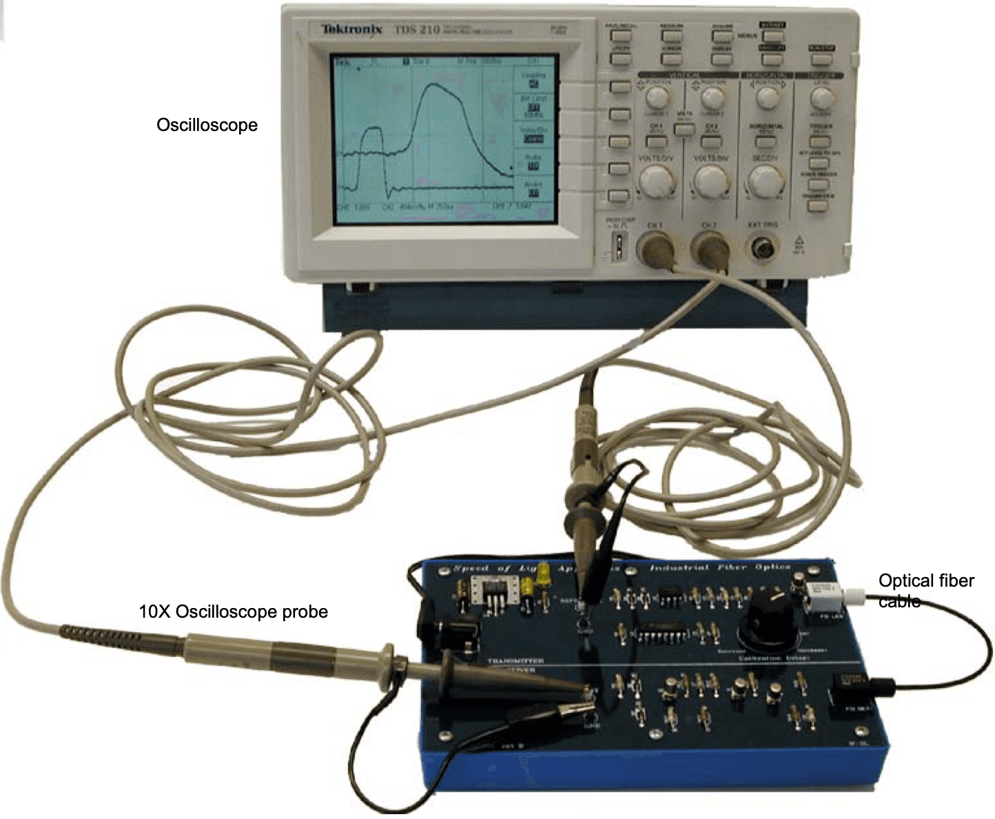
Experimental Methodology: Eliminating Latency

Measuring nanosecond delays requires extreme precision. The main challenge is that our equipment (LEDs photodetectors and BNC cables) introduces its own internal latency ( $\tau_{\text{system}}$ ).

To isolate the signal transit time we employed a Differential Measurement Technique. We compared two different fiber lengths:

Reference Length ( $L_{\text{short}}$ ): 30 cm
Primary Length ( $L_{\text{long}}$ ): 18.9 meters

By subtracting the two results the system latency cancels out perfectly leaving us with the net additional distance: $\Delta L = 18.9\,\text{m} - 0.3\,\text{m} = 18.6\,\text{m}$ .

Schematic of the Time-of-Flight setup — The differential setup used to isolate the 18.6m propagation delay.

Analysis of Results

Using a Digital Storage Oscilloscope (DSO) we observed a temporal shift of $\Delta t \approx 100$ ~ns.

1. Velocity and Refractive Index

Plugging our measured values into the velocity equation: $v_{\exp} = \frac{18.6\,\text{m}}{100 \times 10^{-9}\,\text{s}} = 1.86 \times 10^8\,\text{m/s}$

This yields an experimental refractive index of $n_{\exp} \approx 1.61$ .

2. The Velocity Factor (VF)

A key metric in telecommunications is the Velocity Factor defined as $v_g/c$ . In our case: $\text{VF} = \frac{1.86 \times 10^8}{2.99 \times 10^8} \approx 0.62$ This means light was traveling at 62% of its vacuum speed through our fiber.

Discussion: Why the 10.3% Deviation?

The accepted value for silica is $n \approx 1.46$ . Our value of $1.61$ represents a 10.3% error. In physics the "why" is often more important than the result itself. We identified three major systematic factors:

A. Modal Dispersion and Effective Path Length

Our cable was a multi-mode plastic-clad silica fiber. In multi-mode fibers light follows "zigzag" trajectories. While the physical cable is 18.6m the actual path taken by the light modes is longer. Since we triggered our measurement at the half-maximum point of the pulse we were likely detecting modes that had traveled a significantly longer distance thus inflating our $n_{\exp}$ .

B. Pulse Broadening and Attenuation

As we switched from the 30cm to the 18.9m fiber we observed two things:

The signal amplitude decreased (Attenuation).
The pulse width increased (Broadening).

This is due to Rayleigh Scattering and Material Absorption. The broader pulse makes the "half-maximum" point harder to pin down precisely introducing trigger ambiguity.

Oscilloscope Resolution: Our DSO was set to 50 ns/div. A human error of just 8 ns in cursor placement—hardly a few millimeters on the screen—is enough to account for the entire 10% discrepancy.

Conclusion

This experiment was a practical demonstration of the limitations of high-speed data transmission. While the theoretical speed of light is a constant the effective speed is a slave to waveguide geometry and material properties. For a physics student and developer it’s a reminder that between the code (data) and the hardware (fiber) there's a lot of beautiful messy physics happening.

Technical Specs of the Lab:

Source: Pulsed LED/Laser
Fiber Type: Multi-mode Plastic-Clad Silica (PCS)
Equipment: Digital Storage Oscilloscope (DSO), BNC Interconnects.

References

Goree, J. A. (2002). Experiment S1: Speed of Light – Time of Flight Method. University of Iowa Physics Laboratory Manual.
Agrawal, G. P. (2002). Fiber-Optic Communication Systems (3rd ed.). Wiley-Interscience.
Mohr, P. J., Newell, D. B., & Taylor, B. N. (2018). CODATA Recommended Values of the Fundamental Physical Constants. NIST.
Hecht, E. (2017). Optics (5th ed.). Pearson.
Born, M., & Wolf, E. (1999). Principles of Optics (7th ed.). Cambridge University Press.
Senior, J. M., & Jamro, M. Y. (2009). Optical Fiber Communications: Principles and Practice. Pearson.
Einstein, A. (1905). Zur Elektrodynamik bewegter Körper. Annalen der Physik.